Mahalanobis distance.
One can think of the independent variables (in a regression equation) as defining a multidimensional space in which each observation can be plotted. Also, one can plot a point representing the means for all independent variables. This "mean point" in the multidimensional space is also called the centroid. The Mahalanobis distance is the distance of a case from the centroid in the multidimensional space, defined by the correlated independent variables (if the independent variables are uncorrelated, it is the same as the simple Euclidean distance). Thus, this measure provides an indication of whether or not an observation is an outlier with respect to the independent variable values.
See also, standard residual value, deleted residual and Cook’s distance.
Mann-Scheuer-Fertig Test.
This test, proposed by Mann, Scheuer, and Fertig (1973), is described in detail in, for example, Dodson (1994) or Lawless (1982). The null hypothesis for this test is that the population follows the Weibull distribution with the estimated parameters. Nelson (1982) reports this test to have reasonably good power, and this test can be applied to Type II censored data. For computational details refer to Dodson (1994) or Lawless (1982); the critical values for the test statistic have been computed based on Monte Carlo studies, and have been tabulated for n (sample sizes) between 3 and 25; for n greater than 25, this test is not computed.
The Mann-Scheuer-Fertig test is used in Weibull and Reliability/Failure Time Analysis; see also, Hollander-Proschan Test and Anderson-Darling Test.
Marginal Frequencies.
In a Multi-way table, the values in the margins of the table are simply one-way (frequency) tables for all values in the table. They are important in that they help us to evaluate the arrangement of frequencies in individual columns or rows. The differences between the distributions of frequencies in individual rows (or columns) and in the respective margins inform us about the relationship between the crosstabulated variables.
For more information on Marginal frequencies, see the Crosstabulations section of the Basic Statistics chapter.
Mass.
The term mass in correspondence analysis is used to denote the entries in the two-way table of relative frequencies (i.e., each entry is divided by the sum of all entries in the table). Note that the results from correspondence analysis are still valid if the entries in the table are not frequencies, but some other measure of correspondence, association, similarity, confusion, etc. Since the sum of all entries in the table of relative frequencies is equal to 1.0, one could say that the table of relative frequencies shows how one unit of mass is distributed across the cells of the table. In the terminology of correspondence analysis, the row and column totals of the table of relative frequencies are called the row mass and column mass, respectively.
Manifest Variable.
A manifest variable is a variable that is directly observable or measurable. In path analysis diagrams used in structural modeling (see Path Diagram), manifest variables are usually represented by enclosing the variable name within a square or a rectangle.
Matching Moments Method.
This method can be employed to determine parameter estimates for a distribution (see Quantile- Quantile Plots, Probability-Probability Plots, and Process Analysis). The method of matching moments sets the distribution moments equal to the data moments and solves to obtain estimates for the distribution parameters. For example, for a distribution with two parameters, the first two moments of the distribution (the mean and variance of the distribution, respectively, e.g.,  and
and  , respectively) would be set equal to the first two moments of the data (the sample mean and variance, respectively, e.g., the unbiased estimators x-bar and s**2, respectively) and solved for the parameter estimates. Alternatively, you could use the Maximum Likelihood Method to estimate the parameters. For more information, see Hahn and Shapiro, 1994.
Matrix Plots.
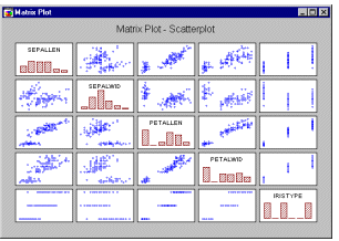
Matrix graphs summarize the relationships between several variables in a matrix of true X-Y plots. The most common type of matrix plot is the scatterplot, which can be considered to be the graphical equivalent of the correlation matrix.
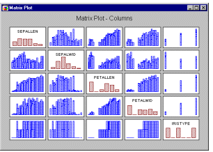
Matrix Plots - Columns.
In this type of Matrix Plot, columns represent projections of individual data points onto the X- axis (showing the distribution of the maximum values), arranged in a matrix format. Histograms representing the distribution of each variable are displayed along the diagonal of the matrix (in square matrices, see example below) or along the edges (in rectangular matrices).
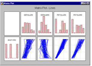
Matrix Plots - Lines.
In this type of Matrix Plot, a matrix of X-Y (i.e., nonsequential) line plots (similar to a scatterplot matrix) is produced in which individual points are connected by a line in the order of their appearance in the data file. Histograms representing the distribution of each variable are displayed along the diagonal of the matrix (in square matrices) or along the edges (in rectangular matrices, see example below).
Matrix Plots - Scatterplot.
In this type of Matrix Plot, 2D Scatterplots are arranged in a matrix format (values of the column variable are used as X coordinates, values of the row variable represent the Y coordinates). Histograms representing the distribution of each variable are displayed along the diagonal of the matrix (in square matrices, see example below) or along the edges (in rectangular matrices).
See also, Data Reduction.
Maximum Likelihood Loss Function.
An common alternative to the least squares loss function is
to maximize the likelihood or log-likelihood function (or to minimize the
negative log-likelihood function; the term maximum likelihood was first
used by Fisher, 1922a). These functions are typically used when fitting
non-linear models. In most general terms, the likelihood function is
defined as:
L=F(Y,Model)= ni=1 { p[yi , Model Parameters(xi)]}
Maximum Likelihood Method.
The method of maximum likelihood (the term first used by Fisher, 1922a) is a general method of estimating parameters of a population by values that maximize the likelihood (L) of a sample. The likelihood L of a sample of n observations x1, x2, ..., xn, is the joint probability function p(x1, x2, ..., xn) when x1, x2, ..., xn are discrete random variables. If x1, x2, ..., xn are continuous random variables, then the likelihood L of a sample of n observations, x1, x2, ..., xn, is the joint density function f(x1, x2, ..., xn).
Let L be the likelihood of a sample, where L is a function of the parameters  1,
1,  2, ...
  k. Then the maximum likelihood estimators of
  1,
1,  2, ...
  k are the values of
  1,
1,  2, ...
  k that maximize L.
Let  be an element of
  . If
. If  is an open interval, and if L(
 ) is differentiable and assumes a maximum on W, then the MLE will be a solution of the following equation: (dL(
 ))/d
))/d = 0. For more information, see Mendenhall and Sincich (1984), Bain and Engelhardt (1989), and Neter, Wasserman, and Kutner (1989).
See also, Nonlinear Estimation or Variance Components and Mixed Model ANOVA/ANCOVA.
Maximum Unconfounding.
Maximum unconfounding is an experimental design criterion that is subsidiary to the criterion of design resolution. The maximum unconfounding criterion specifies that design generators should be chosen such that the maximum number of interactions of less than or equal to the crucial order, given the resolution, are unconfounded with all other interactions of the crucial order. It is an alternative to the minimum aberration criterion for finding the "best" design of maximum resolution. . For discussions of the role of design criteria in experimental design see 2**(k-p) fractional factorial designs and 2**(k-p) Maximally Unconfounded and Minimum Aberration Designs.
MD (Missing data).
Same as Missing values.
Mean.
The mean is a particularly informative measure of the "central tendency" of the variable if it is reported along with its confidence intervals. Usually we are interested in statistics (such as the mean) from our sample only to the extent to which they are informative about the population. The larger the sample size, the more reliable its mean. The larger the variation of data values, the less reliable the mean (see also Elementary Concepts).
Mean = ( xi)/n
xi)/n
where
n is the sample size.
See also, Descriptive Statistics
Mean/S.D.
An algorithm (used in neural networks) to assign linear scaling coefficients for a set of numbers. The mean and standard deviation of the set are found, and scaling factors selected so that these are mapped to desired mean and standard deviation values.
See also Neural Networks.
Mean Substitution of Missing Data.
When you select Mean Substitution, the missing data will be replaced by the means for the respective variables during an analysis.
See also, Casewise vs. pairwise deletion of missing data
Median.
A measure of central tendency, the median (the term first used by Galton, 1882) of a sample is the value for which one-half (50%) of the observations (when ranked) will lie above that value and one-half will lie below that value. When the number of values in the sample is even, the median is computed as the average of the two middle values.
See also, Descriptive Statistics.
Minimax.
An algorithm to assign linear scaling coefficients for a set of numbers. The minimum and maximum of the set are found, and scaling factors selected so that these are mapped to desired minimum and maximum values.
See also, Neural Networks.
Minimum Aberration.
Minimum aberration is an experimental design criterion that is subsidiary to the criterion of design resolution. The minimum aberration design is defined as the design of maximum resolution "which minimizes the number of words in the defining relation that are of minimum length" (Fries & Hunter, 1984). Less technically, the criterion apparently operates by choosing design generators that produce the smallest number of pairs of confounded interactions of the crucial order. For example, the minimum aberration resolution IV design would have the minimum number of pairs of confounded 2-factor interactions. For discussions of the role of design criteria in experimental design see 2**(k-p) fractional factorial designs and 2**(k-p) Maximally Unconfounded and Minimum Aberration Designs.
Missing values.
Values of variables within data sets which are not known. Although such cases that contain missing data are incomplete, they can still be used in data analysis. Various methods exist to substitute missing data (e.g., by mean substitution, various types of interpolations and extrapolations). Also, pariwise deletion of missing data can be used. See also, Pairwise deletion of missing data, Casewise (Listwise) deletion of missing data, Pairwise deletion of missing data vs. mean substitution, and Casewise vs. pairwise deletion of missing data.
Mode.
A measure of central tendency, the mode (the term first used by Pearson, 1895) of a sample is the value which occurrs most frequently in the sample.
See also, Descriptive Statistics.
Monte Carlo.
A computer-intensive technique for assessing how a statistic will perform under repeated sampling. In Monte Carlo methods, the computer uses random number simulation techniques to mimic a statistical population. In the STATISTICA (see University site licenses) Monte Carlo procedure, the computer constructs the population according to the user’s prescription, then does the following:
For each Monte Carlo replication, the computer:
- Simulates a random sample from the population,
- Analyzes the sample,
- Stores the results.
After many replications, the stored results will mimic the sampling distribution of the statistic. Monte Carlo techniques can provide information about sampling distributions when exact theory for the sampling distribution is not available.
MPatt Bar.
Multi-pattern bar plots may be used to represent individual data values of the X variable (the same type of data as in pie charts), however, consecutive data values of the X variable are represented by the heights of sequential vertical bars, each of a different color and pattern (rather than as pie wedges of different widths).
Multidimensional Scaling.
Multidimensional scaling (MDS) can be considered to be an alternative to factor analysis (see Factor Analysis), and it is typically used as an exploratory method. In general, the goal of the analysis is to detect meaningful underlying dimensions that allow the researcher to explain observed similarities or dissimilarities (distances) between the investigated objects. In factor analysis, the similarities between objects (e.g., variables) are expressed in the correlation matrix. With MDS one may analyze not only correlation matrices but also any kind of similarity or dissimilarity matrix (including sets of measures that are not internally consistent, e.g., do not follow the rule of transitivity).
For more information, see the Multidimensional Scaling chapter.
Multilayer Perceptrons.
Feedforward neural networks having linear PSP functions and (usually) non-linear activation functions.
Multimodal Distribution.
A distribution that has multiple modes (thus two or more "peaks").
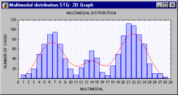
Multimodality of the distribution in a sample is often a strong indication that the distribution of the variable in population is not normal. Multimodality of the distribution may provide important information about the nature of the investigated variable (i.e., the measured quality). For example, if the variable represents a reported preference or attitude, then multimodality may indicate that there are several pronounced views or patterns of response in the questionnaire. Often however, the multimodality may indicate that the sample is not homogenous and the observations come in fact from two or more "overlapping" distributions. Sometimes, multimodality of the distribution may indicate problems with the measurement instrument (e.g, "gage calibration problems" in natural sciences, or "response biases" in social sciences).
See also unimodal distribution, bimodal distribution.
Multiple Dichotomies.
One possible coding scheme that can be used when more than one response is possible from a given question is to code responses using Multiple dichotomies . For example, as part of a larger market survey, suppose you asked a sample of consumers to name their three favorite soft drinks. The specific item on the questionnaire may look like this:
Write down your three favorite soft drinks:
1:__________ 2:__________ 3:__________
Suppose in the above example we were only interested in Coke, Pepsi, and Sprite. One way to code the data in that case would be as follows:
| |
COKE |
PEPSI |
SPRITE |
. . . . |
case 1
case 2
case 3
. . . |
1
. . . |
1
1
. . . |
1
. . . |
|
In other words, one variable was created for each soft drink, then a value of 1 was entered into the respective variable whenever the respective drink was mentioned by the respective respondent. Note that each variable represents a dichotomy; that is, only "1"s and "not 1"s are allowed (we could have entered 1's and 0's, but to save typing we can also simply leave the 0's as blanks or as missing values). When tabulating these variables, we would like to compute the number and percent of respondents (and responses) for each soft drink. In a sense, we "compact" the three variables Coke, Pepsi, and Sprite into a single variable (Soft Drink) consisting of multiple dichotomies.
For more information on Multiple dichotomies, see the Multiple Response Tables section of the Basic Statistics chapter.
Multiple Histogram.
Multiple histograms present frequency distributions of more than one variable in one 2D graph. Unlike the Double-Y Histograms, the frequencies for all variables are plotted against the same left-Y axis.
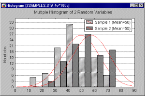
Also, the values of all examined variables are plotted against a single X-axis, which facilitates comparisons between analyzed variables.
Multiple R.
The coefficient of multiple correlation (Multiple R) is the positive square root of R-square (the coefficient of multiple determination, see Residual Variance and R-Square). This statistic is useful in multivariate regression (i.e., multiple independent variables) when you want to describe the relationship between the variables.
Multiple Regression.
The general purpose of multiple regression (the term was first used by Pearson, 1908) is to analyze the relationship between several independent or predictor variables and a dependent or criterion variable.
The computational problem that needs to be solved in multiple regression analysis is to fit a straight line (or plane in an n-dimensional space, where n is the number of independent variables) to a number of points. In the simplest case -- one dependent and one independent variable -- one can visualize this in a scatterplot (scatterplots are two-dimensional plots of the scores on a pair of variables). It is used as either a hypothesis testing or exploratory method.
For more information, see the Multiple Regression chapter.
Multiple Response Variables.
Coding the responses to Multiple response variables is necessary when more than one response is possible from a given question. For example, as part of a larger market survey, suppose you asked a sample of consumers to name their three favorite soft drinks. The specific item on the questionnaire may look like this:
Write down your three favorite soft drinks:
1:__________ 2:__________ 3:__________
Thus, the questionnaires returned to you will contain somewhere between 0 and 3 answers to this item. Also, a wide variety of soft drinks will most likely be named. One way to record the various responses would be to use three multiple response variables and a coding scheme for the many soft drinks. Then we could enter the respective codes (or alphanumeric labels) into the three variables, in the same way that respondents wrote them down in the questionnaire.
| |
Resp. 1 |
Resp. 2 |
Resp. 3 |
case 1
case 2
case 3
. . . |
COKE
SPRITE
PERRIER
. . . |
PEPSI
SNAPPLE
GATORADE
. . . |
JOLT
DR. PEPPER
MOUNTAIN DEW
. . . |
For more information, see the Multiple Response Tables section of the Basic Statistics chapter.
Multiple-response Tables.
Multiple-response tables are Crosstabulation tables used when the categories of interest are not mutually exclusive. Such tables can accommodate Multiple response variables as well as Multiple dichotomies.
For more information, see the Multiple Response Tables section of the Basic Statistics chapter.
Multiplicative Season, Damped Trend.
In this Time Series model, the simple exponential smoothing forecasts are "enhanced" both by a damped trend component (independently smoothed with the single parameter  ; this model is an extension of Brown's one-parameter linear model, see Gardner, 1985, p. 12-13) and a multiplicative seasonal component (smoothed with parameter
  ). For example, suppose we wanted to forecast from month to month the number of households that purchase a particular consumer electronics device (e.g., VCR). Every year, the number of households that purchase a VCR will increase, however, this trend will be damped (i.e., the upward trend will slowly disappear) over time as the market becomes saturated. In addition, there will be a seasonal component, reflecting the seasonal changes in consumer demand for VCR's from month to month (demand will likely be smaller in the summer and greater during the December holidays). This seasonal component may be multiplicative, for example, sales during the December holidays may increase by factor of 1.4 (or 40%) over the average annual sales. To compute the smoothed values for the first season, initial values for the seasonal components are necessary. Also, to compute the smoothed value (forecast) for the first observation in the series, both estimates of S0 and T0 (initial trend) are necessary. These values are computed as:
T0 = (1/ )*Mk-M1)/[(k-1)*p]
where
 is the smoothing parameter
k is the number of complete seasonal cycles
Mk is the mean for the last seasonal cycle
M1 is the mean for the first seasonal cycle
p is the length of the seasonal cycle
and S0 = M1-p*T0/2
Multiplicative Season, Exponential Trend.
In this Time Series model, the simple exponential smoothing forecasts are "enhanced" both by an exponential trend component (independently smoothed with parameter  ) and a multiplicative seasonal component (smoothed with parameter
  ). For example, suppose we wanted to forecast the monthly revenue for a resort area. Every year, revenue may increase by a certain percentage or factor, resulting in an exponential trend in overall revenue. In addition, there could be an multiplicative seasonal component, that is, given the respective annual revenue, each year 20% of the revenue is produced during the month of December, that is, during Decembers the revenue grows by a particular (multiplicative) factor.
To compute the smoothed values for the first season, initial values for the seasonal components are necessary. Also, to compute the smoothed value (forecast) for the first observation in the series, both estimates of S0 and T0 (initial trend) are necessary. By default, these values are computed as:
T0 = exp{[log(Mk)-log(M1)]/p}
where
k is the number of complete seasonal cycles
Mk is the mean for the last seasonal cycle
M1 is the mean for the first seasonal cycle
p is the length of the seasonal cycle
and S0 = exp{log(M1)-p*log(T0)/2}
Multiplicative Season, Linear Trend.
In this Time Series model, the simple exponential smoothing forecasts are "enhanced" both by a linear trend component (independently smoothed with parameter  ) and a multiplicative seasonal component (smoothed with parameter
  ). For example, suppose we were to predict the monthly budget for snow-removal in a community. There may be a trend component (as the community grows, there is an upward trend for the cost of snow removal from year to year). At the same time, there is obviously a seasonal component, reflecting the differential likelihood of snow during different months of the year. This seasonal component could be multiplicative, meaning that given a respective budget figure, it may increase by a factor of, for example, 1.4 during particular winter months; or it may be additive (see above), that is, a particular fixed additional amount of money is necessary during the winter months. To compute the smoothed values for the first season, initial values for the seasonal components are necessary. Also, to compute the smoothed value (forecast) for the first observation in the series, both estimates of S0 and T0 (initial trend) are necessary. By default, these values are computed as:
T0 = (Mk-M1)/((k-1)*p)
where
k is the number of complete seasonal cycles
Mk is the mean for the last seasonal cycle
M1 is the mean for the first seasonal cycle
p is the length of the seasonal cycle
and S0 = M1 - T0/2
Multiplicative Season, No Trend.
This Time Series model is partially equivalent to the simple exponential smoothing model; however, in addition, each forecast is "enhanced" by a multiplicative component that is smoothed independently (see The seasonal smoothing parameter  ). This model would, for example, be adequate when computing forecasts for monthly expected sales for a particular toy. The level of sales may be stable from year to year, or change only slowly; at the same time, there will be seasonal changes (e.g., greater sales during the December holidays), which again may change slowly from year to year. The seasonal changes may affect the sales in a multiplicative fashion, for example, depending on the respective overall level of sales, December sales may always be greater by a factor of 1.4.

© Copyright StatSoft, Inc., 1984-1998
STATISTICA is a trademark of StatSoft, Inc.
 and
and  , respectively) would be set equal to the first two moments of the data (the sample mean and variance, respectively, e.g., the unbiased estimators x-bar and s**2, respectively) and solved for the parameter estimates. Alternatively, you could use the Maximum Likelihood Method to estimate the parameters. For more information, see Hahn and Shapiro, 1994.


 ni=1 { p[yi , Model Parameters(xi)]}
 1,
1,  . If
. If  xi)/n
xi)/n


 ; this model is an extension of Brown's one-parameter linear model, see Gardner, 1985, p. 12-13) and a multiplicative seasonal component (smoothed with parameter
  ). For example, suppose we wanted to forecast from month to month the number of households that purchase a particular consumer electronics device (e.g., VCR). Every year, the number of households that purchase a VCR will increase, however, this trend will be damped (i.e., the upward trend will slowly disappear) over time as the market becomes saturated. In addition, there will be a seasonal component, reflecting the seasonal changes in consumer demand for VCR's from month to month (demand will likely be smaller in the summer and greater during the December holidays). This seasonal component may be multiplicative, for example, sales during the December holidays may increase by factor of 1.4 (or 40%) over the average annual sales. To compute the smoothed values for the first season, initial values for the seasonal components are necessary. Also, to compute the smoothed value (forecast) for the first observation in the series, both estimates of S0 and T0 (initial trend) are necessary. These values are computed as:
 )*Mk-M1)/[(k-1)*p]
 ) and a multiplicative seasonal component (smoothed with parameter