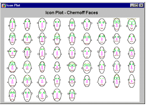
Icon Plots - Chernoff Faces. Chernoff faces is the most "elaborate" type of icon plot. A separate "face" icon is drawn for each case; relative values of the selected variables for each case are assigned to shapes and sizes of individual facial features (e.g., length of nose, angle of eyebrows, width of face).

See also Graphical Analytic Techniques: Icon Plots.
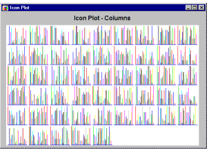
Icon Plots - Columns. In this type of icon plot, an individual column graph is plotted for each case; relative values of the selected variables for each case are represented by the height of consecutive columns.
See also Graphical Analytic Techniques: Icon Plots.
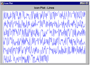
Icon Plots - Lines. In this type of icon plot, an individual line graph is plotted for each case; relative values of the selected variables for each case are represented by the height of consecutive break points of the line above the baseline.
See also Graphical Analytic Techniques: Icon Plots.
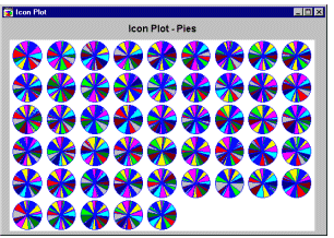
Icon Plots - Pies. In this type of icon plot, data values for each case are plotted as a pie chart (clockwise, starting at 12:00); relative values of selected variables are represented by the size of the pie slices.
See also Graphical Analytic Techniques: Icon Plots.
Icon Plots - Polygons. In this type of icon plot, a separate polygon icon is plotted for each case; relative values of the selected variables for each case are represented by the distance from the center of the icon to consecutive corners of the polygon (clockwise, starting at 12:00).
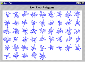
See also Graphical Analytic Techniques: Icon Plots.
Icon Plots - Profiles. In this type of icon plot, an individual area graph is plotted for each case; relative values of the selected variables for each case are represented by the height of consecutive peaks of the profile above the baseline.
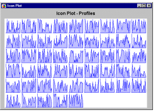
See also Graphical Analytic Techniques: Icon Plots.
Icon Plots - Stars. In this type of icon plot, a separate star-like icon is plotted for each case; relative values of the selected variables for each case are represented (clockwise, starting at 12:00) by the relative length of individual rays in each star. The ends of the rays are connected by a line.
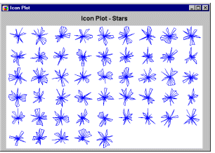
See also Graphical Analytic Techniques: Icon Plots.
Icon Plots - Sun Rays. In this type of icon plot, a separate sun-like icon is plotted for each case; each ray represents one of the selected variables (clockwise, starting at 12:00), and the length of the ray represents 4 standard deviations. Data values of the variables for each case are connected by a line.
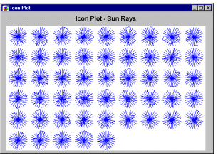
See also Graphical Analytic Techniques: Icon Plots.
Independent vs. Dependent Variables. The terms dependent and independent variable apply mostly to experimental research where some variables are manipulated, and in this sense they are "independent" from the initial reaction patterns, features, intentions, etc. of the subjects. Some other variables are expected to be "dependent" on the manipulation or experimental conditions. That is to say, they depend on "what the subject will do" in response. Independent variables are those that are manipulated whereas dependent variables are only measured or registered.
Somewhat contrary to the nature of this distinction, these terms are also used in studies where we do not literally manipulate independent variables, but only assign subjects to "experimental groups" based on some preexisting properties of the subjects. For example, if in an experiment, males are compared with females regarding their white cell count (WCC), Gender could be called the independent variable and WCC the dependent variable.
See Dependent vs. independent variables for more information.
Inertia. The term inertia in correspondence analysis is used by analogy with the definition in applied mathematics of "moment of inertia," which stands for the integral of mass times the squared distance to the centroid (e.g., Greenacre, 1984, p. 35). Inertia is defined as the total Pearson Chi-square for a two-way frequency table divided by the total sum of all observations in the table.
Interactions. An effect of interaction occurs when a relation between (at least) two variables is modified by (at least one) other variable. In other words, the strength or the sign (direction) of a relation between (at least) two variables is different depending on the value (level) of some other variable(s). (The term interaction was first used by Fisher, 1926). Note that the term "modified" in this context does not imply causality but represents a simple fact that depending on what subset of observations (regarding the "modifier" variable(s)) you are looking at, the relation between the other variables will be different.
For example, imagine that we have a sample of highly achievement-oriented students and another of achievement "avoiders." We now create two random halves in each sample, and give one half of each sample a challenging test, the other an easy test. We measure how hard the students work on the test. The means of this (fictitious) study are as follows:
| Achievement- oriented |
Achievement- avoiders |
|
|---|---|---|
| Challenging Test Easy Test |
10 5 |
5 10 |
How can we summarize these results? Is it appropriate to conclude that (1) challenging tests make students work harder, (2) achievement-oriented students work harder than achievement-avoiders? None of these statements captures the essence of this clearly systematic pattern of means. The appropriate way to summarize the result would be to say that challenging tests make only achievement-oriented students work harder, while easy tests make only achievement-avoiders work harder. In other words, the relation between the type of test and effort is positive in one group but negative in the other group. Thus, the type of achievement orientation and test difficulty interact in their effect on effort; specifically, this is an example of a two-way interaction between achievement orientation and test difficulty. (Note that statements 1 and 2 above would describe so-called main effects.)
For more information regarding interactions, see Interaction Effects in the ANOVA chapter.
Interpolation. Projecting a curve between known data points to infer the value of a function at points between.
Interval Scale. This scale of measurement allows you to not only rank order the items that are measured, but also to quantify and compare the sizes of differences between them (no absolute zero is required).
See also, Measurement scales.
Intraclass Correlation Coefficient. The value of the population intraclass correlation coefficient is a measure of the homogeneity of observations within the classes of a random factor relative to the variability of such observations between classes. It will be zero only when the estimated effect of the random factor is zero and will reach unity only when the estimated effect of error is zero, given that the the total variation of the observations is greater than zero (see Hays, 1988, p. 485).
Note that the population intraclass correlation can be estimated using variance component estimation methods. For more information see the chapter on Variance Components and Mixed-Model ANOVA/ANCOVA.
Invariance Under a Constant Scale Factor (ICSF). A structural model is invariant under a constant scale factor (ICSF) if model fit is not changed if all variables are multiplied by the same constant. Most, but not all, structural models that are of practical interest are ICSF (see Structural Equation Modeling).
Invariance Under Change of Scale (ICS). A structural model is invariant under change of scale if model fit is not changed by rescaling the variables, i.e., by multiplying them by scale factors (see Structural Equation Modeling).
Isotropic Deviation Assignment. An algorithm for assigning radial unit deviations, which selects a single deviation value using a heuristic calculation based on the number of units and the volume of pattern space they occupy, with the objective of ensuring "a reasonable overlap." (Haykin, 1994).
See also the Neural Networks chapter.
JPEG. Acronym for Joint Photographic Experts Group. An ISO/ITU standard for storing images in compressed form using a discrete cosine transform.
Jogging Weights. Adding a small random amount to the weights in a neural network, in an attempt to escape a local optima in error space.
See also the Neural Networks chapter.
Johnson Curves. Johnson (1949) described a system of frequency curves that represents transformations of the standard normal curve (see Hahn and Shapiro, 1967, for details). By applying these transformations to a standard normal variable, a wide variety of non-normal distributions can be approximated, including distributions which are bounded on either one or both sides (e.g., U- shaped distributions). The advantage of this approach is that once a particular Johnson curve has been fit, the normal integral can be used to compute the expected percentage points under the respective curve. Methods for fitting Johnson curves, so as to approximate the first four moments of an empirical distribution, are described in detail in Hahn and Shapiro, 1967, pages 199-220; and Hill, Hill, and Holder, 1976.
See also, Pearson Curves.
JPG. A file name extension used to save JPEG documents (see JPEG).
Kernel functions. Simple functions (typically Gaussians) which are added together, positioned at known data points, to approximate a sampled distribution (Parzen, 1962).
See also the Neural Networks chapter.
K-Means algorithm. An algorithm to assign K centers to represent the clustering of N points (K<N). The points are iteratively adjusted (starting with a random sample of the N points) so that each of the N points is assigned to one of the K clusters, and each of the K clusters is the mean of its assigned points (Bishop, 1995).
See, Cluster Analysis, Neural Networks.
K-Nearest algorithm. An algorithm to assign deviations to radial units. Each deviation is the mean distance to the K-nearest neighbors of the point.
See also, the Neural Networks chapter.
Kohonen Networks. Neural networks based on the topological properties of the human brain, also known as self-organizing feature maps (SOFMs) (Kohonen, 1982; Fausett, 1994; Haykin, 1994; Patterson, 1996).
Kohonen Training. An algorithm which assigns cluster centers to a radial layer by iteratively submitting training patterns to the network, and adjusting the winning (nearest) radial unit center, and its neighbors, towards the training pattern (Kohonen, 1982; Fausett, 1994; Haykin, 1994; Patterson, 1996).
See also, the Neural Networks chapter.
Kurtosis. Kurtosis (the term first used by Pearson, 1905) measures the "peakedness" of a distribution. If the kurtosis is clearly different than 0, then the distribution is either flatter or more peaked than normal; the kurtosis of the normal distribution is 0. Kurtosis is computed as:
Kurtosis = [n*(n+1)*M4 - 3*M2*M2*(n-1)]/[(n-1)*(n-2)*(n-3)* 4]
4]
where:
Mj is equal to:  (xi-Meanx)j
n is the valid number of cases
 4 is the standard deviation (sigma) raised to the fourth power
See also, Descriptive Statistics.
