Y = a + b₁*X₁ + b₂*X₂ + ... +b_p*X_p

Note that in this equation, the regression coefficients (or B coefficients) represent the independent contributions of each independent variable to the prediction of the dependent variable. However, their values may not be comparable between variables because they depend on the units of measurement or ranges of the respective variables. Some software products will produce both the raw regression coefficients (B coefficients) and the Beta coefficients (note that the Beta coefficients are comparable across variables).

See also, the Multiple Regression chapter.

Back Propagation. A training algorithm for multilayer perceptrons. Reliable and well-known, although significantly slower than some of the more modern algorithms (see Patterson, 1996; Fausett, 1994; Haykin, 1994).

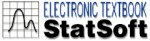
Bar/Column Plots, 2D. The Bar/Column Plot represents sequences of values as bars or columns (one case is represented by one bar/column). If more than one variable is selected, each plot can be represented in a separate graph or all of them can be combined in one display as multivariate clusters of bars/columns (one cluster per case, see example below).

Bar Dev Plot. The "bar deviation" plot is similar to the Bar X plot, in that individual data points are represented by vertical bars, however, the bars connect the data points to a user-selectable baseline. If the baseline value is different than the plot's Y-axis minimum, then individual bars will extend either up or down, depending on the direction of the "deviation" of individual data points from the baseline.

Bar Left Y Plot. In this plot, one horizontal bar is drawn for each data point (i.e., each pair of XY coordinates, see example below), connecting the data point and the left Y-axis. The vertical position of the bar is determined by the data point's Y value, and its length by the respective X value.

Bar Right Y Plot. In this plot, one horizontal bar is drawn for each data point (i.e., each pair of XY coordinates), connecting the data point and the right Y-axis. The vertical position of the bar is determined by the data point's Y value, and its length by the respective X value.

Bar Top Plot. (Also known as "hanging" column plots.) In this plot, one vertical bar is drawn for each data point (i.e., each pair of XY coordinates), connecting the data point and the upper X-axis. The horizontal position of the bar is determined by the data point's X value, and its length by the respective Y value.

Bar X Plot. In this plot, one vertical bar is drawn for each data point (i.e., each pair of XY coordinates), connecting the data point and the lower X-axis.

The horizontal position of the bar is determined by the data point's X value, and its height by the respective Y value.

Bartlett Window. In Time Series, the Bartlett window is a weighted moving average transformation used to smooth the periodogram values. In the Bartlett window (Bartlett, 1950) the weights are computed as:

w_j = 1-(j/p)    (for j = 0 to p)
w_-j = w_j    (for j 0)

where p = (m-1)/2

This weight function will assign the greatest weight to the observation being smoothed in the center of the window, and increasingly smaller weights to values that are further away from the center.

See also, Basic Notations and Principles.

Batch algorithms in STATISTICA Neural Networks. Algorithms which calculate the average gradient over an epoch, rather than adjusting on a case-by-case basis during training. Quick propagation, Delta-Bar-Delta, conjugate gradient descent and Levenberg-Marquardt are all batch algorithms.

Bayesian Networks. Networks based on Bayes' theorem, on the inference of probability distributions from data sets.

See also, probabilistic and generalized regression neural networks.

Best Network Retention. A facility (implemented in STATISTICA Neural Networks) to automatically store the best neural network discovered during training, for later restoration at the end of a set of experiments.

See also the chapter on Neural Networks.

Beta Coefficients. The Beta coefficients are the regression coefficients you would have obtained had you first standardized all of your variables to a mean of 0 and a standard deviation of 1. Thus, the advantage of Beta coefficients (as compared to B coefficients which are not standardized) is that the magnitude of these Beta coefficients allow you to compare the relative contribution of each independent variable in the prediction of the dependent variable.

See also, the Multiple Regression chapter.

Beta Distribution. The beta distribution (the term first used by Gini, 1911) is defined as:

f(x) = (+)/(()()) * x^-1 * (1-x)^-1
0 x 1
> 0, > 0

where
        (gamma) is the Gamma function
,    are the shape parameters

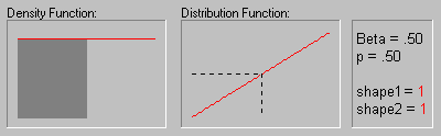
The animation above shows the beta distribution as the two shape parameters change.

Bimodal Distribution. A distribution that has two modes (thus two "peaks").

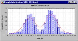
Bimodality of the distribution in a sample is often a strong indication that the distribution of the variable in population is not normal. Bimodality of the distribution may provide important information about the nature of the investigated variable (i.e., the measured quality). For example, if the variable represents a reported preference or attitude, then bimodality may indicate a polarization of opinions. Often however, the bimodality may indicate that the sample is not homogenous and the observations come in fact from two or more "overlapping" distributions. Sometimes, bimodality of the distribution may indicate problems with the measurement instrument (e.g, "gage calibration problems" in natural sciences, or "response biases" in social sciences).

See also unimodal distribution, multimodal distribution.

Binomial Distribution. The binomial distribution (the term first used by Yule, 1911) is defined as:

f(x) = [n!/(x!*(n-x)!)] * p^x * q^n-x
for x = 0, 1, 2, ..., n

where
p     is the probability of success at each trial
q     is equal to 1-p
n     is the number of independent trials

Bivariate Normal Distribution. Two variables follow the bivariate normal distribution if for each value of one variable, the corresponding values of another variable are normally distributed. The bivariate normal probability distribution function for a pair of continuous random variables (X and Y) is given by:

f(x,y) = {1/[212 * (1-)1/2]} * exp[-1/2(1-2)] * {[(x-1)/1]2 -

2[(x-1)/1] * [(y-2)/2] + [(y-2)/2]2}

- < x < , - < y < , - < 1 < , - < 2 < , 1 > 0, 2 > 0, and -1 < < 1

where
₁, ₂    are the respective means of the random variables X and Y
₁, ₂   are the respective standard deviations of the random variables X and Y
           is the correlation coefficient of X and Y
e             is the base of the natural logarithm, sometimes called Euler's e (2.71...)
          is the constant Pi (3.14...)

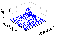
See also, Normal Distribution, Elementary Concepts (Normal Distribution)

For some problems (for example a Heywood Case in factor analysis), it may be possible to reduce the discrepancy function by estimating a variance to be a negative number. In that case, the program does "the best it can" within the permissible parameter space, but does not actually obtain the "global minimum" of the discrepancy function.

Box Plot/Medians (Block Stats Graphs). This type of Block Stats Graph will produce a box plot of medians (and min/max values and 25th and 75th percentiles) for the columns or rows of the block. Each box will represent data from one column or row.

Box Plot/Means (Block Stats Graphs). This type of Block Stats Graph will produce a box plot of means (and standard errors and standard deviations) for the columns or rows of the block. Each box will represent data from one column or row.

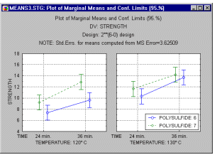
Box Plots, 2D. In Box Plots (this term was first used by Tukey, 1970), ranges or distribution characteristics of values of a selected variable (or variables) are plotted separately for groups of cases defined by values of a categorical (grouping) variable. The central tendency (e.g., median or mean), and range or variation statistics (e.g., quartiles, standard errors, or standard deviations) are computed for each group of cases and the selected values are presented in the selected box plot style. Outlier data points can also be plotted.

Box Plots, 2D - Box Whiskers. This type of box plot will place a box around the midpoint (i.e., mean or median) which represents a selected range (i.e., standard error, standard deviation, min-max, or constant) and whiskers outside of the box which also represent a selected range (see the example graph, below).

Box Plots, 2D - Boxes. This type of box plot will place a box around the midpoint (i.e., mean or median) which represents the selected range (i.e., standard error, standard deviation, min-max, or constant).

Box Plots, 2D - Whiskers. In this style of box plot, the range (i.e., standard error, standard deviation, min-max, or constant) is represented by "whiskers" (i.e., as a line with a serif on both ends, see graph below).

Box Plots, 3D. In Box Plots (this term was first used by Tukey, 1970), ranges or distribution characteristics of values of selected variables are plotted separately for groups of cases defined by values of a categorical (grouping) variable. The central tendency (e.g., median or mean), and range or variation statistics (e.g., quartiles, standard errors, or standard deviations) are computed for each group of cases and the selected values are presented in the selected box plot style. Outlier data points can also be plotted.

Box Plots 3D - Border-style Ranges. In this style of 3D Sequential Box Plot, the ranges of values of selected variables are plotted separately for groups of cases defined by values of a categorical (grouping) variable. The central tendency (e.g., median or mean), and range or variation statistics (e.g., quartiles, standard errors, or standard deviations) are computed for each variable and for each group of cases and the selected values are presented as points with "whiskers," and the ranges marked by the "whiskers" are connected with lines (i.e., range borders) separately for each variable.

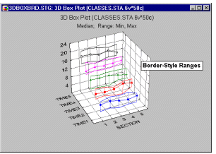
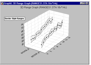
3D Range plots (see example graph below) differ from 3D Box plots in that for Range plots, the ranges are the values of the selected variables (e.g., one variable contains the minimum range values and another variable contains the maximum range values) while for Box plots, the ranges are calculated from variable values (e.g., standard deviations, standard errors, or min-max value).

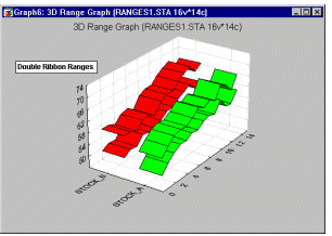
Box Plots 3D - Double Ribbon Ranges. In this style of 3D Sequential Box Plot, the ranges of values of selected variables are plotted separately for groups of cases defined by values of a categorical (grouping) variable. The range or variation statistics (e.g., quartiles, standard errors, or standard deviations) are computed for each variable and for each group of cases and the selected values are presented as double ribbons.

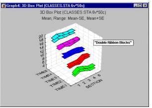
3D Range plots (see example graph below) differ from 3D Box plots in that for Range plots, the ranges are the values of the selected variables (e.g., one variable contains the minimum range values and another variable contains the maximum range values) while for Box plots the ranges are calculated from variable values (e.g., standard deviations, standard errors, or min-max value).

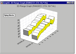
Box Plots 3D - Flying Blocks. In this style of 3D Sequential Box Plot, the ranges of values of selected variables are plotted separately for groups of cases defined by values of a categorical (grouping) variable. The central tendency (e.g., median or mean), and range or variation statistics (e.g., quartiles, standard errors, or standard deviations) are computed for each variable and for each group of cases and the selected values are presented as "flying" blocks.

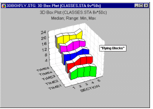
3D Range plots (see example graph below) differ from 3D Box plots in that for Range plots, the ranges are the values of the selected variables (e.g., one variable contains the minimum range values and another variable contains the maximum range values) while for Box plots the ranges are calculated from variable values (e.g., standard deviations, standard errors, or min-max value).

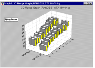
Box Plots 3D - Flying Boxes. In this style of 3D Sequential Box Plot, the ranges of values of selected variables are plotted separately for groups of cases defined by values of a categorical (grouping) variable. The central tendency (e.g., median or mean), and range or variation statistics (e.g., quartiles, standard errors, or standard deviations) are computed for each variable and for each group of cases and the selected values are presented "flying" boxes.

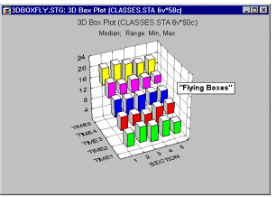
3D Range plots (see example graph below) differ from 3D Box plots in that for Range plots, the ranges are the values of the selected variables (e.g., one variable contains the minimum range values and another variable contains the maximum range values) while for Box plots the ranges are calculated from variable values (e.g., standard deviations, standard errors, or min-max value).

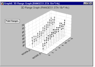
Box Plots 3D - Points. In this style of 3D Sequential Box Plot, the ranges of values of selected variables are plotted separately for groups of cases defined by values of a categorical (grouping) variable. The central tendency (e.g., median or mean), and range or variation statistics (e.g., quartiles, standard errors, or standard deviations) are computed for each variable and for each group of cases and the selected values are presented as point markers connected by a line.

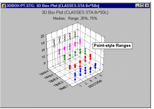
3D Range plots (see example graph below) differ from 3D Box plots in that for Range plots, the ranges are the values of the selected variables (e.g., one variable contains the minimum range values and another variable contains the maximum range values) while for Box plots, the ranges are calculated from variable values (e.g., standard deviations, standard errors, or min-max value).

Box-Ljung Q Statistic. In Time Series analysis, you can shift a series by a given lag k. For that given lag, the Box-Ljung Q statistic is defined by:

Q_k = n*(n+2)*Sum(r_i²/(n-1))
for i = 1 to k

When the number of observations is large, then the Q statistic has a Chi- square distribution with k-p-q degrees of freedom, where p and q are the number of autoregressive and moving average parameters, respectively.

Breakdowns. Breakdowns are procedures which allow us to calculate descriptive statistics and correlations for dependent variables in each of a number of groups defined by one or more grouping (independent) variables. It is used as either a hypothesis testing or exploratory method.

For more information, see the Breakdowns section in the Basic Statistics chapter.

Brushing. Perhaps the most common and historically first widely used technique explicitly identified as graphical exploratory data analysis is brushing, an interactive method allowing one to select on-screen specific data points or subsets of data and identify their (e.g., common) characteristics, or to examine their effects on relations between relevant variables (e.g., in scatterplot matrices) or to identify (e.g., label) outliers. For more information on brushing, see Special Topics in Graphical Analytic Techniques: Brushing.

Burt Table. Multiple correspondence analysis expects as input (i.e., the program will compute prior to the analysis) a so-called Burt table. The Burt table is the result of the inner product of a design or indicator matrix. If you denote the data (design or indicator matrix) as matrix X, then matrix product X'X is a Burt table); shown below is an example of a Burt table that one might obtain in this manner.

	SURVIVAL		AGE			LOCATION
	NO	YES	<50	50-69	69+	TOKYO	BOSTON	GLAMORGN
SURVIVAL:NO SURVIVAL:YES   AGE:UNDER_50 AGE:A_50TO69 AGE:OVER_69  LOCATION:TOKYO LOCATION:BOSTON LOCATION:GLAMORGN	210 0   68 93 49   60 82 68	0 554   212 258 84   230 171 153	68 212   280 0 0   151 58 71	93 258   0 351 0   120 122 109	49 84   0 0 133   19 73 41	60 230   151 120   19   290     0     0	82 171     58 122   73       0 253     0	68 153     71 109   41       0     0 221

Overall, the data matrix is symmetrical. In the case of 3 categorical variables (as shown above), the data matrix consists 3 x 3 = 9 partitions, created by each variable being tabulated against itself, and against the categories of all other variables. Note that the sum of the diagonal elements in each diagonal partition (i.e., where the respective variables are tabulated against themselves) is constant (equal to 764 in this case). The off-diagonal elements in each partition in this example are all 0. If the cases in the design or indicator matrix are assigned to categories via fuzzy coding, then the off- diagonal elements of the diagonal partitions are not necessarily equal to 0.