See also, Basic Notations and Principles.

Data Mining. StatSoft defines data mining as an analytic process designed to explore large amounts of (typically business or market related) data in search for consistent patterns and/or systematic relationships between variables, and then to validate the findings by applying the detected patterns to new subsets of data.

Data mining uses many of the principles and techniques traditionally referred to as Exploratory Data Analysis (EDA). For more information, see Data Mining.

Data Reduction. The term Data Reduction is used in two distinctively different meanings:

Data Reduction by decreasing the dimensionality (exploratory multivariate statistics). This interpretation of the term Data Reduction pertains to analytic methods (typically multivariate exploratory techniques such as Factor Analysis, Multidimensional Scaling, Cluster Analysis, Canonical Correlation, or Neural Networks) that involve reducing the dimensionality of a data set by extracting a number of underlying factors, dimensions, clusters, etc., that can account for the variability in the (multidimensional) data set. For example, in poorly designed questionnaires, all responses provided by the participants on a large number of variables (scales, questions, or dimensions) could be explained by a very limited number of "trivial" or artifactual factors. For example, two such underlying factors could be: (1) the respondent's attitude towards the study (positive or negative) and (2) the "social desirability" factor (a response bias representing a tendency to respond in a socially desirable manner).

Data Reduction by unbiased decreasing of the sample size (exploratory graphics). This type of Data Reduction is applied in exploratory graphical data analysis of extremely large data sets. The size of the data set can obscure an existing pattern (especially in large line graphs or scatterplots) due to the density of markers or lines. Then, it can be useful to plot only a representative subset of the data (so that the pattern is not hidden by the number of point markers) to reveal the otherwise obscured but still reliable pattern. For an animated illustration, see the Data Reduction section of the Selected Topics in Graphical Analytic Techniques chapter.

Data Rotation (in 3D space). Changing the viewpoint for 3D scatterplots (e.g., simple, spectral, or space plots) may prove to be an effective exploratory technique since it can reveal patterns that are easily obscured unless you look at the "cloud" of data points from an appropriate angle (see the animation below).

Rotating or spinning a 3D graph will allow you to find the most informative location of the "viewpoint" for the graph. For more information see the section on Data Rotation (in 3D space) in the Graphical Techniques chapter.

Data Warehousing. StatSoft defines data warehousing as a process of organizing the storage of large, multivariate data sets in a way that facilitates the retrieval of information for analytic purposes.

For more information, see Data Warehousing.

Deleted residual. The deleted residual is the residual value for the respective case, had it not been included in the regression analysis, that is, if one would exclude this case from all computations. If the deleted residual differs greatly from the respective standardized residual value, then this case is possibly an outlier because its exclusion changed the regression equation.

See also, standard residual value, Mahalanobis distance, and Cook’s distance.

Delta-Bar-Delta. A heuristic modification to the back propagation neural networks algorithm, which attempts to automatically adjust the learning rate along each dimension of search space to match the search space topology (Jacobs, 1988; Patterson, 1996).

Derivative-free Function Minimization Algorithms. Nonlinear Estimation offers several general function minimization algorithms that follow different search strategies which do not depend on the second-order derivatives. These strategies are sometimes very effective for minimizing loss functions with local minima.

Desirability Profiles. The relationship between predicted responses on one or more dependent variables and the desirability of responses is called the desirability function. Profiling the desirability of responses involves, first, specifying the desirability function for each dependent variable, by assigning predicted values a score ranging from 0 (very undesirable) to 1 (very desirable). The individual desirability scores for the predicted values for each dependent variable are then combined by computing their geometric mean. Desirability profiles consist of a series of graphs, one for each independent variable, of overall desirability scores at different levels of one independent variable, holding the levels of the other independent variables constant at specified values. Inspecting the desirability profiles can show which levels of the predictor variables produce the most desirable predicted responses on the dependent variables.

For a detailed description of response/desirability profiling see Profiling Predicted Responses and Response Desirability.

Detrended Probability Plots. This type of graph is used to evaluate the normality of the distribution of a variable, that is, whether and to what extent the distribution of the variable follows the normal distribution. The selected variable will be plotted in a scatterplot against the values "expected from the normal distribution." This plot is constructed in the same way as the standard normal probability plot, except that before the plot is generated, the linear trend is removed. This often "spreads out" the plot, thereby allowing the user to detect patterns of deviations more easily.

Deviation. In radial units, a figure multiplied by the radial exemplar's squared distance from the input pattern to generate the unit's activation level, before submission to the activation function. See neural networks.

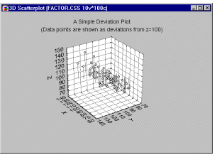
Deviation Plots 3D. Data (representing the X, Y, and Z coordinates of each point) in this type of graph are represented in 3D space as "deviations" from a specified base-level of the Z-axis.

Deviation plots are similar to space plots. As compared to space plots, however in deviation plots the "deviations plane" is "invisible" and not marked by the location of the X-Y axes (those axes are always fixed in the standard bottom position). Deviation plots may help explore the nature of 3D data sets by displaying them in the form of deviations from arbitrary (horizontal) levels. Such "cutting" methods can help identify interactive relations between variables.

See also, Data Rotation (in 3D space) in the Graphical Techniques chapter.

DFFITS. Several measures have been given for testing for leverage and influence of a specific case in regression (including studentized residuals, studentized deleted residuals, DFFITS, and standardized DFFITS). Belsley et al. (1980) have suggested DFFITS, a measure which gives greater weight to outlying observations than Cook's distance. The formula for DFFITS is

DFFIT_i = _ie_i/(1-_i)

where
e_i    is the error for the ith case
h_i    is the leverage for the ith case

and _i = 1/N + h_i.

For more information see Hocking (1996) and Ryan (1997).

Differencing (in Time Series). In this Time Series transformation, the series will be transformed as: X=X-X(lag). After differencing, the resulting series will be of length N-lag (where N is the length of the original series).

Dimensionality Reduction. Data Reduction by decreasing the dimensionality (exploratory multivariate statistics). This interpretation of the term Data Reduction pertains to analytic methods (typically multivariate exploratory techniques such as Factor Analysis, Multidimensional Scaling, Cluster Analysis, Canonical Correlation, or Neural Networks) that involve reducing the dimensionality of a data set by extracting a number of underlying factors, dimensions, clusters, etc., that can account for the variability in the (multidimensional) data set. For more information, see Data Reduction.

Discrepancy Function. A numerical value that expresses how badly a structural model reproduces the observed data. The larger the value of the discrepancy function, the worse (in some sense) the fit of model to data. In general, the parameter estimates for a given model are selected to make a discrepancy function as small as possible.

The discrepancy functions employed in structural modeling all satisfy the following basic requirements:

1. They are non-negative, i.e., always greater than or equal to zero.
2. They are zero only if fit is perfect, i.e., if the model and parameter estimates perfectly reproduce the observed data.
3. The discrepancy function is a continuous function of the elements of S, the sample covariance matrix, and (), the "reproduced" estimate of S obtained by using the parameter estimates and structural model.

Discriminant Function Analysis. Discriminant function analysis is used to determine which variables discriminate between two or more naturally occurring groups (it is used as either a hypothesis testing or exploratory method). For example, an educational researcher may want to investigate which variables discriminate between high school graduates who decide (1) to go to college, (2) to attend a trade or professional school, or (3) to seek no further training or education. For that purpose the researcher could collect data on numerous variables prior to students' graduation. After graduation, most students will naturally fall into one of the three categories. Discriminant Analysis could then be used to determine which variable(s) are the best predictors of students' subsequent educational choice (e.g., IQ, GPA, SAT).

For more information, see the Discriminant Function Analysis chapter; see also the Classification Trees chapter.

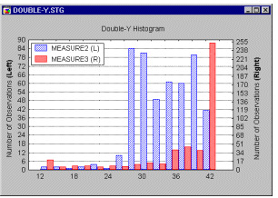
Double-Y Histograms. The Double-Y histogram can be considered to be a combination of two separately scaled multiple histograms. Two different series of variables can be selected. A frequency distribution for each of the selected variables will be plotted but the frequencies of the variables entered into the first list (called Left-Y variables) will be plotted against the left-Y axis, whereas the frequencies of the variables entered into the second list (called Right-Y variables) will be plotted against the right-Y axis. The names of all variables from the two lists will be included in the legend followed by a letter L or R, denoting the Left-Y and Right-Y axis, respectively.

This graph is useful to compare distributions of variables with different frequencies.