*(t - 0.5)/m]}
(for t=0 to m-1)
*(t - 0.5)/m]}
(for t=0 to m-1)wt = 0.5*{1-cos[
*(N - t + 0.5)/m]}
(for t=N-m to N-1)
wt = 0.5*{1-cos[*(t - 0.5)/m]}
(for t=0 to m-1)
wt = 0.5*{1-cos[*(N - t + 0.5)/m]}
(for t=N-m to N-1)
where m is chosen so that 2*m/N is equal to the proportion of data to be tapered (p).
Ternary Plots, 2D - Scatterplot. In this type of ternary graph, the triangular coordinate systems are used to plot three (or more) variables [the components X, Y, and Z] in two dimensions. Here, the points representing the proportions of the component variables (X, Y, and Z) are plotted.
See also, Data Reduction.
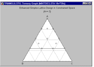
Ternary Plots, 3D. A ternary plot can be used to examine relations between four or more dimensions where three of those dimensions represent components of a mixture (i.e., the relations between them is constrained such that the values of the three variables add up to the same constant). One typical application of this graph is when the measured response(s) from an experiment depends on the relative proportions of three components (e.g., three different chemicals) which are varied in order to determine an optimal combination of those components (e.g., in mixture designs).
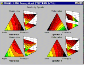
Ternary Plots, 3D - Categorized Scatterplot. The responses associated with the proportions of the component variables (X, Y, and Z) in a ternary graph are plotted in a 3-dimensional display for each level of the grouping variable (or user-defined subset of data). One component graph is produced for each level of the grouping variable (or user-defined subset of data) and all the component graphs are arranged in one display to allow for comparisons between the subsets of data (categories).
See also, Data Reduction.
Ternary Plots, 3D - Categorized Space. In this type of ternary graph, 3D scatterplot data are represented through the use of an X-Y- Z plane (defined via a triangular coordinate system) positioned at a user-selectable level of the vertical V-axis (which "sticks up" through the middle of the plane) and categorized by each level of the grouping variable (or user-defined subset of data). One component graph is produced for each level of the grouping variable (or user-defined subset of data) and all the component graphs are arranged in one display to allow for comparisons between the subsets of data (categories).
The level of the X-Y-Z plane can be adjusted in order to divide the X-Y-Z-V space into meaningful parts (e.g., featuring different patterns of the relation between the three variables).
Ternary Plots, 3D - Categorized Surface. A surface is fit to a four-coordinate data set in this 3-dimensional ternary graph categorized by each level of the grouping variable (or user-defined subset of data). One component graph is produced for each level of the grouping variable (or user-defined subset of data) and all the component graphs are arranged in one display to allow for comparisons between the subsets of data (categories).
Ternary Plots, 3D - Categorized Trace. In this type of ternary graph, you can examine the relations between four or more dimensions (X, Y, Z, and V1, V2, etc.) as a 3D trace plot categorized by each level of the grouping variable (or user-defined subset of data). One component graph is produced for each level of the grouping variable (or user-defined subset of data) and all the component graphs are arranged in one display to allow for comparisons between the subsets of data (categories).
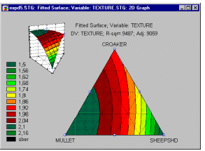
Ternary Plots, 3D - Contour/Areas. In this type of ternary graph, the 3-dimensional surface (fitted to a four-coordinate data set) is projected onto a 2-dimensional plane as an area contour.
Ternary Plots, 3D - Contour/Lines. In this type of ternary graph, the 3-dimensional surface (fitted to a four-coordinate data set) is projected onto a 2-dimensional plane as a line contour (see graph below).
Ternary Plots, 3D - Deviation. This type of ternary graph allows you to examine the relations between four or more dimensions (X, Y, Z, and V1, V2, etc.) as "deviations" from a specified base-level of the V- axis where three of those dimensions (X, Y, and Z) represent components of a mixture (i.e., the relations between them is constrained such that the values of the three variables add up to the same constant for each case).
Ternary Plots, 3D - Space. This type of ternary graph offers a distinctive method of representing 3D scatterplot data through the use of an X-Y-Z plane (defined via a triangular coordinate system) positioned at a user-selectable level of the vertical V-axis (which "sticks up" through the middle of the plane). The level of the X-Y-Z plane can be adjusted in order to divide the X-Y-Z- space into meaningful parts (e.g., featuring different patterns of the relation between the three variables).
THAID. THAID is a classification trees program developed by Morgan & Messenger (1973) that performs multi-level splits when computing classification trees. For discussion of the differences of THAID from other classification tree programs, see A Brief Comparison of Classification Tree Programs.
Threshold. A criterion value (sometimes arbitrarily established) that is used to determine if particular conditions are met or a point separating conditions. (In neural networks, a value subtracted from the weighted sum in a linear PSP unit to produce the activation level. In radial units, the threshold is actually treated as a deviation.)
Time Series. A Time series is a sequence of measurements, typically taken at successive points in time. Time series analysis includes a broad spectrum of exploratory and hypothesis testing methods that have two main goals: (a) identifying the nature of the phenomenon represented by the sequence of observations, and (b) forecasting (predicting future values of the time series variable). Both of these goals require that the pattern of observed time series data is identified and more or less formally described. Once the pattern is established, we can interpret and integrate it with other data (i.e., use it in our theory of the investigated phenomenon, e.g., seasonal commodity prices). Regardless of the depth of our understanding and the validity of our interpretation (theory) of the phenomenon, we can extrapolate the identified pattern to predict future events.
For more information, see the Time Series chapter.
Time-Dependent Covariates. Time-dependent covariates occur when the effect of the covariate on survival is dependent on time (i.e., the conditional hazard at each point in time is a function of the covariate and time).
Tolerance (in Multiple Regression). The tolerance of a variable is defined as 1 minus the squared multiple correlation of this variable with all other independent variables in the regression equation. Therefore, the smaller the tolerance of a variable, the more redundant is its contribution to the regression (i.e., it is redundant with the contribution of other independent variables). If the tolerance of any of the variables in the regression equation is equal to zero (or very close to zero), then the regression equation cannot be evaluated (the matrix is said to be ill-conditioned, and it cannot be inverted).
Topological Map. The radial layer of a Kohonen network, with units laid out in two-dimensions, and trained so that inter-related clusters tend to be situated close together in the layer. Used for cluster analysis (Kohonen, 1982; Fausett, 1994; Haykin, 1994; Patterson, 1996). See, Neural Networks.
Trace Plots 3D. As in 3D Scatterplots, each data point in Trace Plots is represented by its location in 3D space as determined by the values of the variables selected as X, Y, and Z (and interpreted as the X, Y, and Z axis coordinates). The data points are then connected sequentially (in the order encountered in the data file) with a line to form a "trace" of a sequential process (e.g., movement, change of a phnomenon over time, etc.).
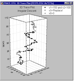
A good metaphor of the information that is best represented in a trace plot is that of the trajectory of an object in three-dimensional space.
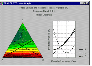
Trace Plot, Categorized (Ternary Graph). This type of ternary graph allows you to examine the relations between four or more dimensions (X, Y, Z, and V1, V2, etc.) as a 3D trace plot where three of those dimensions (X, Y, and Z) represent components of a mixture (i.e., the relations between them is constrained such that the values of the three variables add up to the same constant for each case). Data points in this graph are positioned as in regular 3D scatterplots, however, individual data points are connected with a line (in the order in which they were read from the data file), visualizing a "trace" of sequential values.
Trimmed Means. For certain graphs (e.g., 2D Box Plots, 3D Box Plots, Categorized Box Plots), an option is available to trim the extreme values from the distribution of values of a variable. For example, you can trim (i.e., remove) the lowest 5% and the highest 5% from the distribution of values. The mean of the trimmed distribution of values is referred to as a "trimmed mean" (this term was first used by Tukey, 1962).
Tukey Window. In Time Series, the Tukey window is a weighted moving average transformation used to smooth the periodogram values. In the Tukey (Blackman and Tukey, 1958) or Tukey-Hanning window (named after Julius Von Hann), for each frequency, the weights for the weighted moving average of the periodogram values are computed as:
wj = 0.5 + 0.5*cos(*j/p) (for j=0 to p)
w-j = wj (for j  0)
0)
where p = (m-1)/2x.
This weight function will assign the greatest weight to the observation being smoothed in the center of the window, and increasingly smaller weights to values that are further away from the center.
See also, Spectrum Analysis - Basic Notations and Principles.
Two-State in Neural Networks. An encoding technique for nominal variables with only two values, where the nominal variable is represented by a single input or output unit, either set or cleared. See, Neural Networks.
Type I and II Censoring. So-called Type I censoring describes the situation when a test is terminated at a particular point in time, so that the remaining items are only known not to have failed up to that time (e.g., we start with 100 light bulbs, and terminate the experiment after a certain amount of time). In this case, the censoring time is often fixed, and the number of items failing is a random variable. In Type II censoring the experiment would be continued until a fixed proportion of items have failed (e.g., we stop the experiment after exactly 50 light bulbs have failed). In this case, the number of items failing is fixed, and time is the random variable.
Data sets with censored observations can be analyzed via Survival Analysis or via Weibull and Reliability/Failure Time Analysis. See also, Single and Multiple Censoring and Left and Right Censoring.
Type I Error Rate (Alpha). The probability of incorrectly rejecting a true statistical null hypothesis.
For more information see the chapter on Power Analysis.