Odds Ratio.
The odds ratio is useful in the interpretation of the results of Logistic regression (see Neter, Wasserman, and Kutner, 1989) and is computed from a 2x2 classification table which displays the predicted and observed classification of cases for a binary dependent variable:
(f11 * f22)/(f12 * f21)
where fij represents the respective frequencies in the 2x2 table.
On-Line Analytic Processing (OLAP) (or Fast Analysis of Shared Multidimensional Information - FASMI).
The term On-Line Analytic Processing refers to technology that allows users of multidimensional data bases to generate on-line descriptive or comparative summaries ("views") of data and other analytic queries.
For more information, see On-Line Analytic Processing (OLAP); see also, Data Warehousing and Data Mining techniques.
One-of-N Encoding in Neural Networks.
Representing a nominal variable using a set of input or output units, one unit for each possible nominal value. During training, one of the units will be on and the others off. See, Neural Networks.
One-Off in Neural Networks.
A case typed in and submitted to the neural network as a one-off procedure (not part of a data set, and not used in training). See, Neural Networks.
Operating characteristic curves, for quality control charts.
A common supplementary plot to standard quality control charts is the so-called operating characteristic or OC curve. One question that comes to mind when using standard variable or attribute charts is how sensitive is the current quality control procedure? Put in more specific terms, how likely is it that you will not find a sample (e.g., a mean in an X-bar chart) outside the control limits (i.e., accept the production process as "in control"), when, in fact, it has shifted by a certain amount? This probability is usually referred to as the b (beta) error probability, that is, the probability of erroneously accepting a process (mean, mean proportion, mean rate defectives, etc.) as being "in control."
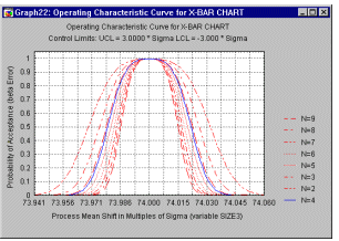 Operating characteristic curves are extremely useful for exploring the power of the quality control procedure. The actual decision concerning sample sizes should depend not only on the cost of implementing the plan (e.g., cost per item sampled), but also on the costs resulting from not detecting quality problems. The OC curve allows the engineer to estimate the probabilities of not detecting shifts of certain sizes in the production quality.
For more information, see also Operating Characteristic Curves.
Ordinal Scale.
The ordinal scale of measurement represents the ranks of a variable's values. Values measured on an ordinal scale contain information about their relationship to other values only in terms of whether they are "greater than" or "less than" other values but not in terms of "how much greater" or "how much smaller."
See also, Measurement scales.
Outer Arrays.
In Taguchi experimental design methodology, the repeated measurements of the response variable are often taken in a systematic fashion, with the goal to manipulate noise factors. The levels of those factors are then arranged in a so-called outer array, i.e., an (orthogonal) experimental design. However, usually the repeated measurements are placed in separate columns in the data spreadsheet (i.e., each is a different variable); thus the index i (in the formulas for smaller-the-better, larger-the-better, and signed target) runs across the columns or variables in the data spreadsheet, or the levels of the factors in the outer array.
See Signal-to-Noise (S/N) Ratios for more details.
Outliers.
Outliers are atypical (by definition), infrequent observations; data points which do not appear to follow the characteristic distribution of the rest of the data. These may reflect genuine properties of the underlying phenomenon (variable), or be due to measurement errors or other anomalies which should not be modeled.
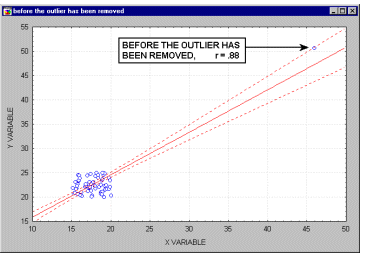
Because of the way in which the regression line is determined in Multiple Regression (especially the fact that it is based on minimizing not the sum of simple distances but the sum of squares of distances of data points from the line), outliers have a profound influence on the slope of the regression line (see the animation below) and consequently on the value of the correlation coefficient. A single outlier is capable of considerably changing the slope of the regression line and, consequently, the value of the correlation. Note, that as shown on that
illustration, just one outlier can be entirely responsible for a high value of the correlation that otherwise (without the outlier) would be close to zero. Needless to say, one should never base important conclusions on the value of the correlation coefficient alone (i.e., examining the respective scatterplot is always recommended).
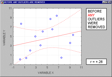
Note that if the sample size is relatively small, then including or excluding specific data points that are not as clearly "outliers" as the one shown in the previous example may have a profound influence on the
regression line (and the correlation coefficient). This is illustrated in the following example where we call the points being excluded "outliers;" one may argue, however, that they are not outliers but rather extreme values.
Typically, we believe that outliers represent a random error that we would like to be able to control. Needless to say, outliers may not only artificially increase the value of a correlation coefficient, but they can also decrease the value of a "legitimate" correlation.
See also Confidence Ellipse.
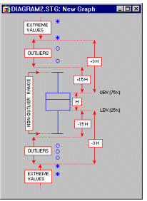
Outliers (in Box Plots).
Values which are "far" from the middle of the distribution are referred to as outliers and extreme values if they meet certain conditions.
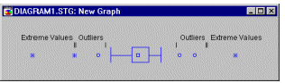
A data point is deemed to be an outlier if the following conditions hold:
data point value > UBV + *o.c.*(UBV - LBV)
or
data point value < LBV - *o.c.*(UBV - LBV)
where
UBV is the upper value of the box in the box plot (e.g., the mean + standard error or the 75th percentile).
LBV is the lower value of the box in the box plot (e.g., the mean - standard error or the 25th percentile).
o.c. is the outlier coefficient.
For example, the following diagram illustrates the ranges of outliers and extremes in the "classic" box and whisker plot (for more information about box plots, see Tukey, 1977).
Overfitting.
When attempting to fit a curve to a set of data points, producing a curve with high curvature which fits the data points well, but does not model the underlying function well, its shape being distorted by the noise inherent in the data.
See also, Neural Networks.
Overlearning in Neural Networks.
When an iterative training algorithm is run, overfitting which occurs when the algorithm is run for too long (and the network is too complex for the problem or the available quantity of data).
See also, Neural Networks.
© Copyright StatSoft, Inc., 1984-1998
STATISTICA is a trademark of StatSoft, Inc.